pacman::p_load(tidytext, widyr, wordcloud, DT, ggwordcloud, textplot, lubridate, hms,
tidyverse, tidygraph, ggraph, igraph)Hands-on_Ex05
Visualising and Analysing Text Data with R: tidytext methods
Getting Started
Installing and launching R packages
Importing Multiple Text Files from Multiple Folders
Creating a folder list
news20 <- "data/20news/"Define a function to read all files from a folder into a data frame
read_folder <- function(infolder) {
  tibble(file = dir(infolder,
                    full.names = TRUE)) %>%
    mutate(text = map(file,
                      read_lines)) %>%
    transmute(id = basename(file),
              text) %>%
    unnest(text)
}
Importing Multiple Text Files from Multiple Folders
Reading in all the messages from the 20news folder
raw_text <- tibble(folder =
                     dir(news20,
                         full.names = TRUE)) %>%
  mutate(folder_out = map(folder,
                          read_folder)) %>%
  unnest(cols = c(folder_out)) %>%
  transmute(newsgroup = basename(folder),
            id, text)
write_rds(raw_text, "data/20news.rds")
Initial EDA
news20 <- read_rds("data/news20.rds")

raw_text <- news20
raw_text %>%
  group_by(newsgroup) %>%
  summarize(messages = n_distinct(id)) %>%
  ggplot(aes(messages, newsgroup)) +
  geom_col(fill = "lightblue") +
  labs(y = NULL)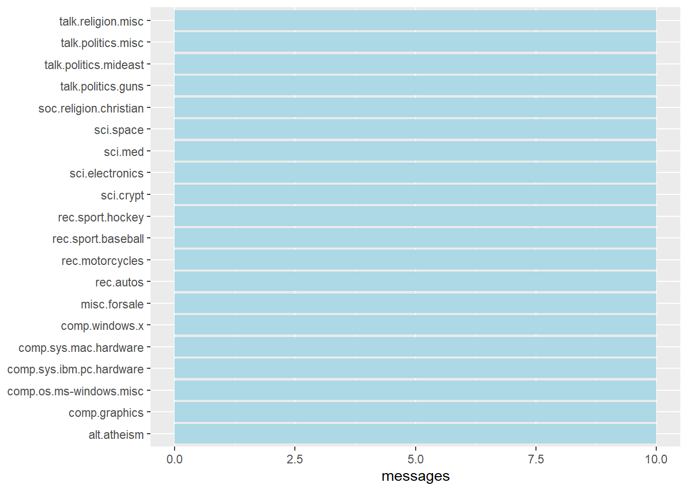
Introducing tidytext
Removing header and automated email signitures
cleaned_text <- raw_text %>%
  group_by(newsgroup, id) %>%
  filter(cumsum(text == "") > 0,
         cumsum(str_detect(
           text, "^--")) == 0) %>%
  ungroup()
Removing lines with nested text representing quotes from other users.
cleaned_text <- cleaned_text %>%
  filter(str_detect(text, "^[^>]+[A-Za-z\\d]")
         | text == "",
         !str_detect(text,
                     "writes(:|\\.\\.\\.)$"),
         !str_detect(text,
                     "^In article <")
  )
Text Data Processing
usenet_words <- cleaned_text %>%
  unnest_tokens(word, text) %>%
  filter(str_detect(word, "[a-z']$"),
         !word %in% stop_words$word)

usenet_words %>%
  count(word, sort = TRUE)
# A tibble: 5,542 × 2
word n
<chr> <int>
1 people 57
2 time 50
3 jesus 47
4 god 44
5 message 40
6 br 27
7 bible 23
8 drive 23
9 homosexual 23
10 read 22
# ℹ 5,532 more rowswords_by_newsgroup <- usenet_words %>%
count(newsgroup, word, sort = TRUE) %>%
ungroup()Visualising Words in newsgroups
wordcloud(words_by_newsgroup$word,
          words_by_newsgroup$n,
          max.words = 300)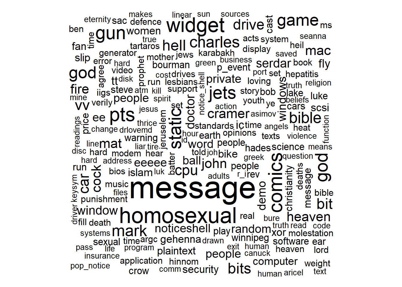
Visualising Words in newsgroups
# set.seed(1234)
#
# words_by_newsgroup %>%
#   filter(n > 0) %>%
# ggplot(aes(label = word,
#           size = n)) +
#   geom_text_wordcloud() +
#   theme_minimal() +
#   facet_wrap(~newsgroup)
Basic Concept of TF-IDF
Computing tf-idf within newsgroups
tf_idf <- words_by_newsgroup %>%
  bind_tf_idf(word, newsgroup, n) %>%
  arrange(desc(tf_idf))
Visualising tf-idf as interactive table
DT::datatable(tf_idf, filter = 'top') %>%
  formatRound(columns = c('tf', 'idf',
                          'tf_idf'),
              digits = 3) %>%
  formatStyle(0,
              target = 'row',
              lineHeight='25%')
Visualising tf-idf as interactive table
DT::datatable(tf_idf, filter = 'top') %>%
  formatRound(columns = c('tf', 'idf',
                          'tf_idf'),
              digits = 3) %>%
  formatStyle(0,
              target = 'row',
              lineHeight='25%')
Visualising tf-idf within newsgroups
tf_idf %>%
  filter(str_detect(newsgroup, "^sci\\.")) %>%
  group_by(newsgroup) %>%
  slice_max(tf_idf,
            n = 12) %>%
  ungroup() %>%
  mutate(word = reorder(word,
                        tf_idf)) %>%
  ggplot(aes(tf_idf,
             word,
             fill = newsgroup)) +
  geom_col(show.legend = FALSE) +
  facet_wrap(~ newsgroup,
             scales = "free") +
  labs(x = "tf-idf",
       y = NULL)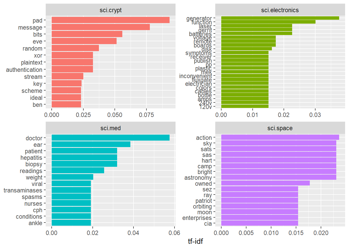
Counting and correlating pairs of words with the widyr package
newsgroup_cors <- words_by_newsgroup %>%
  pairwise_cor(newsgroup,
               word,
               n,
               sort = TRUE)
isualising correlation as a network
set.seed(2017)

newsgroup_cors %>%
  filter(correlation > .025) %>%
  graph_from_data_frame() %>%
  ggraph(layout = "fr") +
  geom_edge_link(aes(alpha = correlation,
                     width = correlation)) +
  geom_node_point(size = 6,
                  color = "lightblue") +
  geom_node_text(aes(label = name),
                 color = "red",
                 repel = TRUE) +
  theme_void()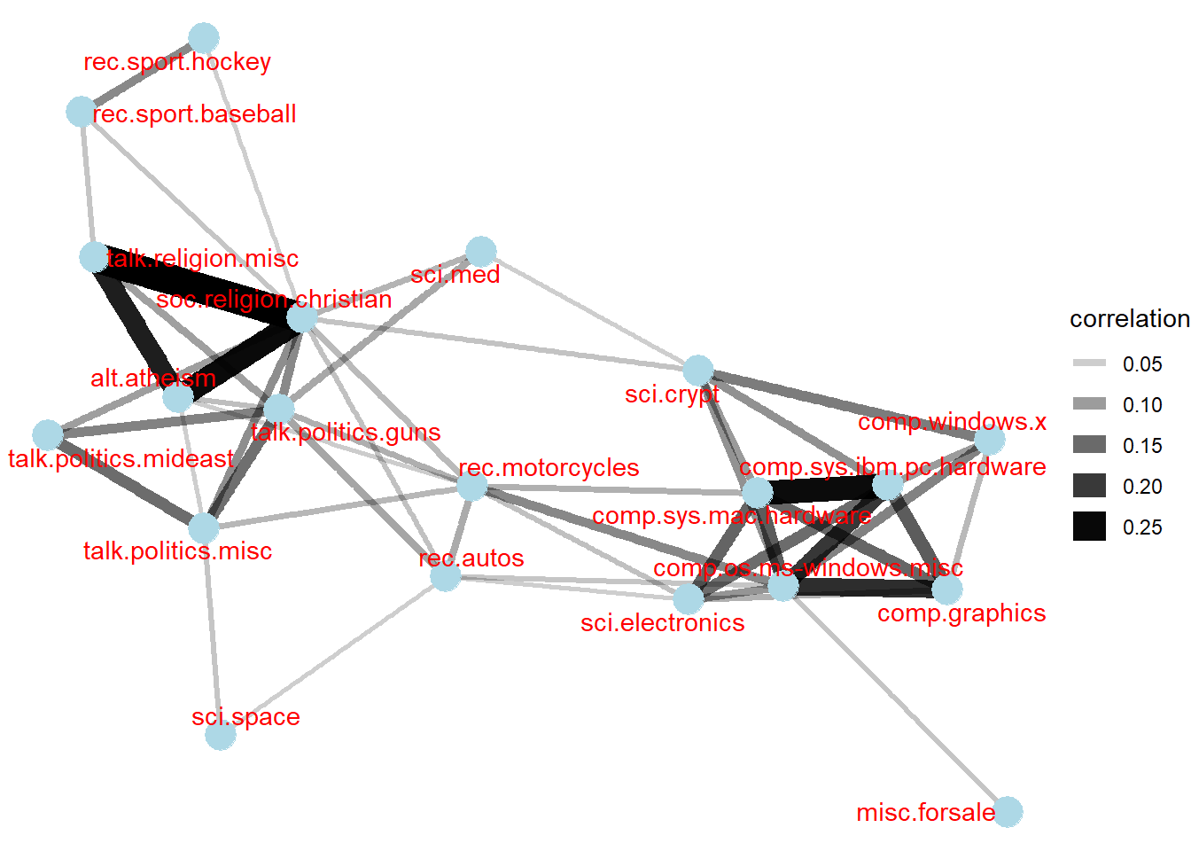
Bigram
bigrams <- cleaned_text %>%
  unnest_tokens(bigram,
                text,
                token = "ngrams",
                n = 2)

bigrams
# A tibble: 28,827 × 3
newsgroup id bigram
<chr> <chr> <chr>
1 alt.atheism 54256 <NA>
2 alt.atheism 54256 <NA>
3 alt.atheism 54256 as i
4 alt.atheism 54256 i don't
5 alt.atheism 54256 don't know
6 alt.atheism 54256 know this
7 alt.atheism 54256 this book
8 alt.atheism 54256 book i
9 alt.atheism 54256 i will
10 alt.atheism 54256 will use
# ℹ 28,817 more rowsCounting bigrams
bigrams_count <- bigrams %>%
  filter(bigram != 'NA') %>%
  count(bigram, sort = TRUE)

bigrams_count
# A tibble: 19,888 × 2
bigram n
<chr> <int>
1 of the 169
2 in the 113
3 to the 74
4 to be 59
5 for the 52
6 i have 48
7 that the 47
8 if you 40
9 on the 39
10 it is 38
# ℹ 19,878 more rowsCleaning bigram
bigrams_separated <- bigrams %>%
  filter(bigram != 'NA') %>%
  separate(bigram, c("word1", "word2"),
           sep = " ")

bigrams_filtered <- bigrams_separated %>%
  filter(!word1 %in% stop_words$word) %>%
  filter(!word2 %in% stop_words$word)

bigrams_filtered
# A tibble: 4,607 × 4
newsgroup id word1 word2
<chr> <chr> <chr> <chr>
1 alt.atheism 54256 defines god
2 alt.atheism 54256 term preclues
3 alt.atheism 54256 science ideas
4 alt.atheism 54256 ideas drawn
5 alt.atheism 54256 supernatural precludes
6 alt.atheism 54256 scientific assertions
7 alt.atheism 54256 religious dogma
8 alt.atheism 54256 religion involves
9 alt.atheism 54256 involves circumventing
10 alt.atheism 54256 gain absolute
# ℹ 4,597 more rowsCounting the bigram again
bigram_counts <- bigrams_filtered %>%
  count(word1, word2, sort = TRUE)
Create a network graph from bigram data frame
bigram_graph <- bigram_counts %>%
  filter(n > 3) %>%
  graph_from_data_frame()
bigram_graph
IGRAPH f8a55d1 DN-- 40 24 --
+ attr: name (v/c), n (e/n)
+ edges from f8a55d1 (vertex names):
[1] 1 ->2 1 ->3 static ->void
[4] time ->pad 1 ->4 infield ->fly
[7] mat ->28 vv ->vv 1 ->5
[10] cock ->crow noticeshell->widget 27 ->1993
[13] 3 ->4 child ->molestation cock ->crew
[16] gun ->violence heat ->sink homosexual ->male
[19] homosexual ->women include ->xol mary ->magdalene
[22] read ->write rev ->20 tt ->ee Visualizing a network of bigrams with ggraph
set.seed(1234)

ggraph(bigram_graph, layout = "fr") +
  geom_edge_link() +
  geom_node_point() +
  geom_node_text(aes(label = name),
                 vjust = 1,
                 hjust = 1)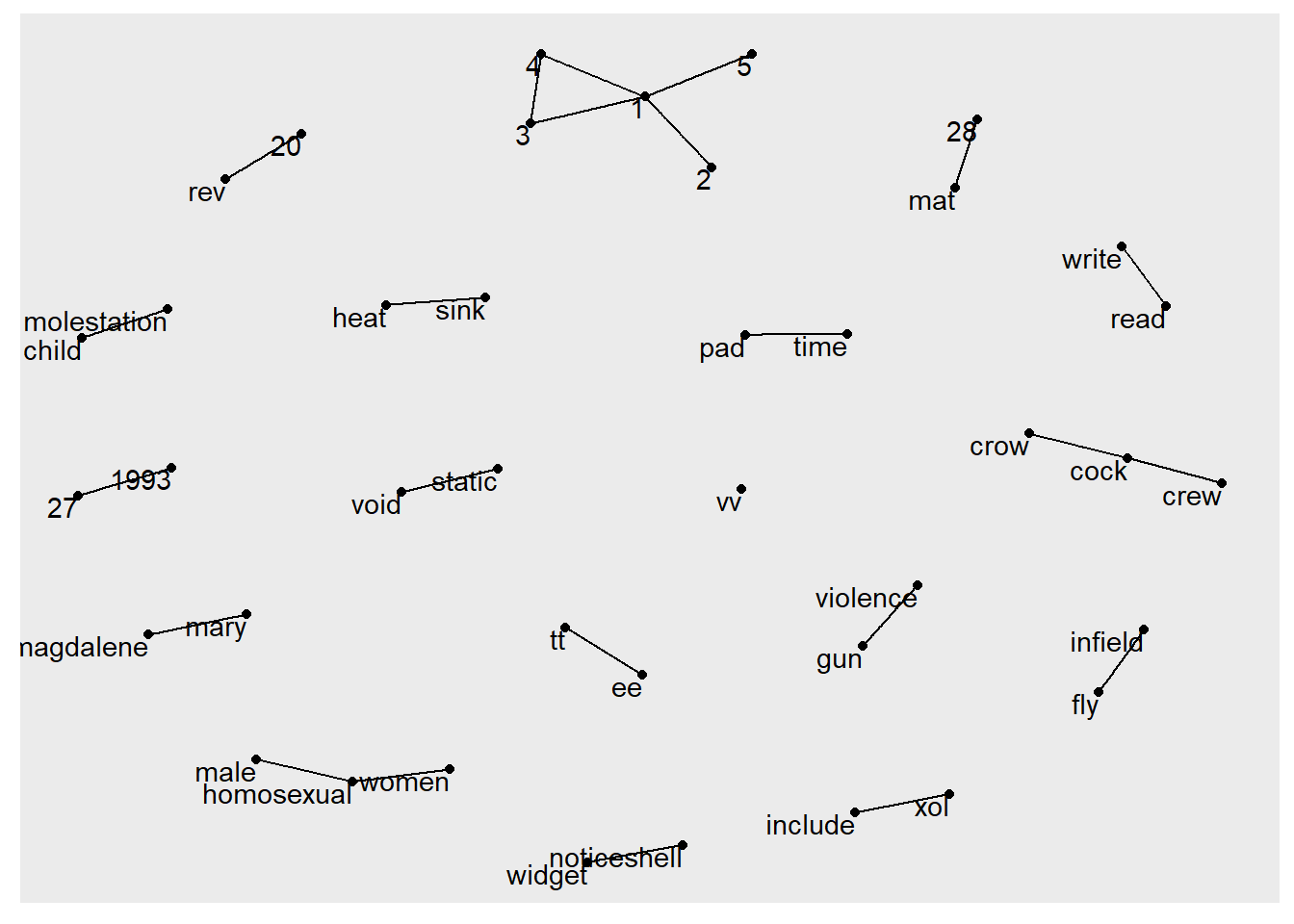
Revised version
set.seed(1234)

a <- grid::arrow(type = "closed",
                 length = unit(.15,
                               "inches"))

ggraph(bigram_graph,
       layout = "fr") +
  geom_edge_link(aes(edge_alpha = n),
                 show.legend = FALSE,
                 arrow = a,
                 end_cap = circle(.07,
                                  'inches')) +
  geom_node_point(color = "lightblue",
                  size = 5) +
  geom_node_text(aes(label = name),
                 vjust = 1,
                 hjust = 1) +
  theme_void()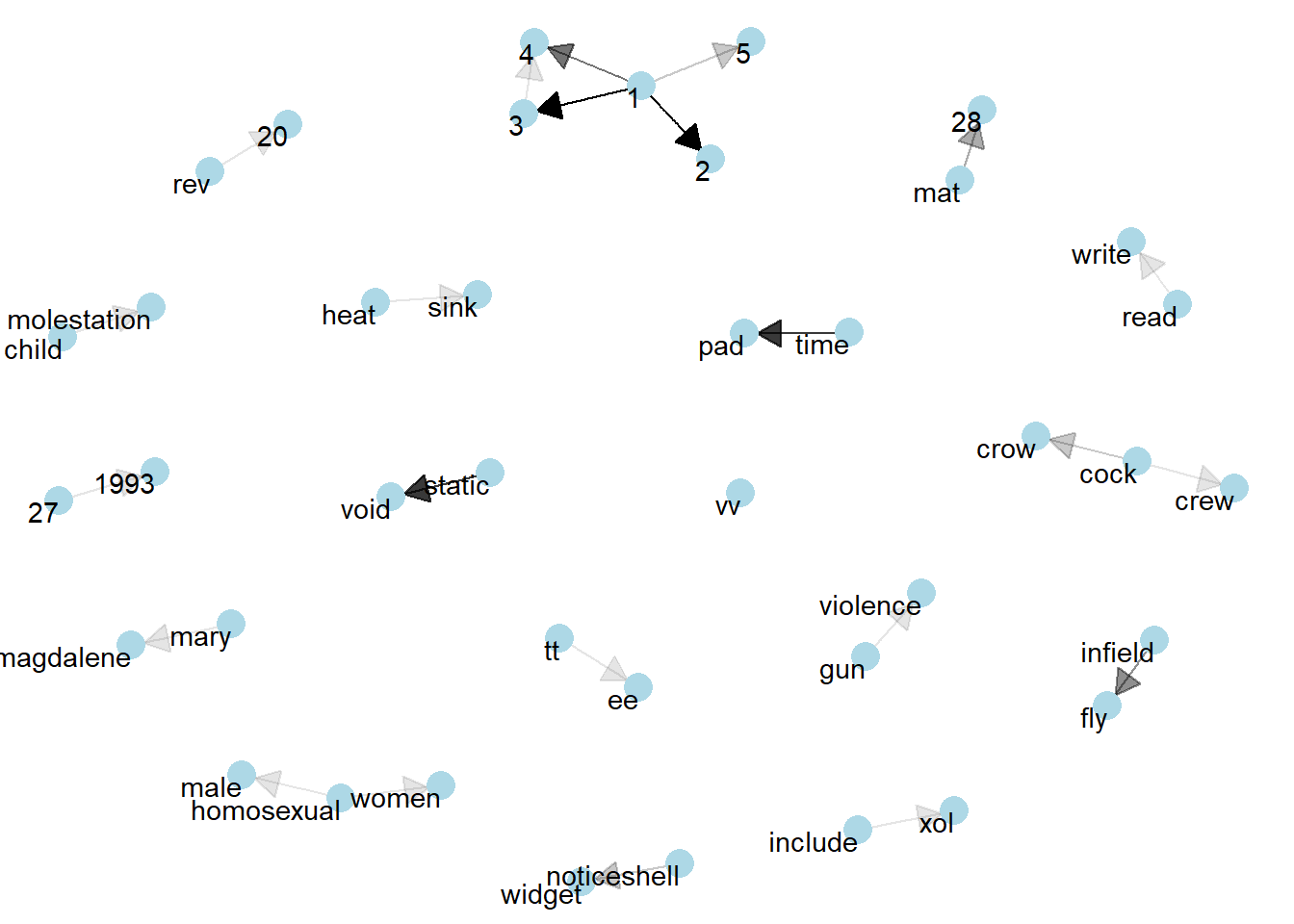
References
Reference guide widyr: Widen, process, and re-tidy a dataset United Nations Voting Correlations